In some spatial group atlas articles, we often see a picture, which
is to calculate the complexity of cells in a region. We take an article
published in Cell this year as an example to see how to calculate the
complexity of cells in a region. The name of the article is Single-cell
spatial transcriptome reveals cell-type organization in the macaque
cortex, and the link to the article is: https://linkinghub.elsevier.com/retrieve/pii/S0092867423006797,
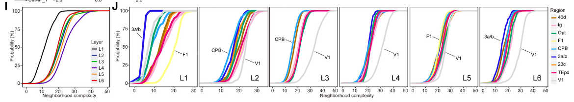
there is such a picture in Figure II:
The meaning of I figure is the complexity distribution of each cell
in different layers. The calculation of each cell's complexity is to
take each cell as the center, 200 pixels as the radius, draw a circle,
and calculate the number of cell types different from this cell in this
circle. According to this understanding, we can write the program.
1
2
3
4
5
6
7
8
9
10
# first is the introduction of the package
import anndata as ad
import numpy as np
import pandas as pd
import scanpy as sc
from matplotlib.ticker import FuncFormatter
import seaborn as sns
import numpy as np
from collections import Counter
import matplotlib.pyplot as plt
here I wrote three functions, the calculation speed of the three
functions is faster than one, but the degree of understanding is more
difficult than one
# the first function is the most common one we understand to traverse all cells defcalculate_neighborhood_complexity(cell_coordinates, cluster_labels, radius): neighborhood_complexities = []
for central_cell, central_cluster_label inzip(cell_coordinates, cluster_labels): complexity = 0
# and the second function uses some numpy functions, which is much faster than the first function defcalculate_neighborhood_complexity(cell_coordinates, cluster_labels, radius): unique_labels, label_indices = np.unique(cluster_labels, return_inverse=True) complexity_counts = np.zeros(len(cell_coordinates), dtype=int) for i, central_cell inenumerate(cell_coordinates): distances = np.linalg.norm(cell_coordinates - central_cell, axis=1) mask = np.logical_and(distances > 0, distances <= radius) previous_complexities = set() for cell_idx, cluster_idx inenumerate(label_indices[mask]): if cluster_idx notin previous_complexities: complexity_counts[i] += 1 previous_complexities.add(cluster_idx) total_cells = len(cell_coordinates) complexity_probabilities = np.bincount(complexity_counts) / total_cells return complexity_counts, complexity_probabilities
# and the third function uses KD tree, which maintains the edge when building the tree, and the speed is much faster than the second function from scipy.spatial import cKDTree
# Build a KD-tree from the cell coordinates kdtree = cKDTree(cell_coordinates)
for i, central_cell inenumerate(cell_coordinates): # Query the KD-tree to find the cell indices within the radius neighbor_indices = kdtree.query_ball_point(central_cell, radius) previous_complexities = set()
for cell_idx, cluster_idx inzip(neighbor_indices, label_indices[neighbor_indices]): if cluster_idx notin previous_complexities: complexity_counts[i] += 1 previous_complexities.add(cluster_idx)
# adata is the data of the spatial group
# obs region is the information of the brain region
# obs celltype is the information of cell type
# obsm spatial is the coordinate information of cells
# layer is the information of each layer
# The measured speed is about 15 min for the first function for 20k cells, about 5s for the second function, and about 1.5s for the third function